Instructor: Sigurd B. Angenent
TA: Joshua Rushton.
Lecture: 1:20MWF in room 224 Ingraham Hall.
Grades: The course grade will be based on two midterm exams, the final exam, and your discussion section grade. In total you can get 100 points: 20 per midterm, 20 from your discussion section, and 40 from the final exam. The total scores will then be curved. (Past experience shows that one needs roughly(!) 85 points or more to get an A, while at least 55 points are usually needed to score above an F.) The precise curve will NOT be determined until after the final exam.
Exams: There will be two midterm exams. These will be 50 minute exams held in class, and at the usual lecture time.
The first midterm will be held on February 21.
The second midterm will be held on March 30.
Final exam: 07:45 A.M. Tuesday May 10. Towards the end of the semester the location of most final exams can be found on the registrar's website.
Office hours are by appointment. Contact me after class if you want to see me and we can pick a time.
Homework will be assigned by Josh.
Topics to be covered in this semester.
Differential Calculus
Review of differential calculus of functions of several variables: the Chain rule, wave equation, Laplacian in polar coordinates.
Integral Calculus
Line integrals, Potential functions for vector fields, Exact differential equations.
Multiple integrals: definition and some applications. The transformation formula, and integrals in polar, cylindrical and spherical coordinates.
Green's theorem.
Surfaces
Parametrized surfaces, surface area, normal vectors.
Surface integrals, change of parameter
Theorems of Stokes and Gauss (and Ostrogradski). Applications: Dirichlet's principle, Dulac's test, incompressible fluid flow.
Differential Equations — Linear Systems with Constant Coefficients
Definition and computation of etA for a square matrix A. The Cayley–Hamilton theorem. Variation of constants.
And, what really happened:
Jan 19 I derived the equation for the vibrating string, aka the one-dimensional wave equation. See §9.4 of our book for the equation. Next time I'll show how to find all solutions of the wave equation.
You should try to solve problems 8 and 9 from §9.3, and 2, 3 from §9.5. Then try your hand at these problems. I'll do the case A=1, B=0, C=c2 in the next lecture so you may want to wait until then.
Jan 21 I showed how to transform the wave equation
ftt-c2fxx=0 into the easier
equation guv=0.
I also made a start on line integrals (see §10 in the book).
Jan 24 §§10.4, 10.6. Definition and examples of Line Integrals:
independence of the parametrization (Theorem 10.1, p.327). Interpretation
as “work.” Kinetic energy of a motion.
Suggested problems: §10.5: 1, 2(draw the curve!), 5, 6, 9, 12 (draw
the curves and surfaces mentioned in the problem).
Jan 26 Line integral w.r.t arclength(§10.7).
The 2nd Fundamental Theorem for line integrals (§ 10.11)
— Reconstructing a function from its gradient.
The 1st Fundamental Theorem for line integrals (§ 10.14)
— when is a vector field a gradient?
We looked at the line integral ∫ydx along various curves. I posed
the following problem: Interpret the line integral ∫ydx along the
following two curves in terms of areas of regions in the drawing.
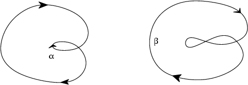
Jan 28 I stated a theorem on when a vector field is a gradient.
More precise versions of the theorem I stated in class are in
§10.15&16, theorems 10.5 and 10.6. The example following that is
partially in the book as example 2 on page 341.
I also mentioned the definition of a connected set. See §10.10.
Problems to do: § 10.13– 1a,d,e,f (draw S in each
case),
2 (done in class), 3, 4, 5a, 6a (a vector field is
“conservative” if it is the gradient of some function),10
§10.18 – 13,14.
Have a careful look at problems 17&18 (page 346). Draw the set
T. Instead of doing these two problems you could compute the partial
derivatives of θ by implicit differentiation. The angle
θ in polar coordinates satisfies
F(x,y,θ)= y cos θ - x sin θ = 0.
Use this to compute ∂θ/∂x and ∂θ/∂y.
Jan 31 Our next subject is the Riemann integral for functions on
Rn. While recalling the definition of the integral for functions
of one variable it turned out that the concepts of “supremum”
and “infimum” need to be explained first.
Here is a link to brief notes
with some exercises & solutions on the least upper and greatest
lower bounds of sets of real numbers.
Feb 2,4 I presented the definition of the Riemann integral of a function on a rectangle, and showed that it coincides with the iterated integral
∫∫R f = ∫ab (∫cd f(x,y)dy)dx
I proved that a continuous function on a rectangle is bounded, and stated
the theorem which says that every continuous function on a rectangle is
Riemann-integrable.
All theory presented so far is covered in §§11.1–10.
Being able to compute double integrals is an important skill, so you should
try problems §11.9:1—14.
Feb 7 We finish the section on multiple integrals by introducing the concept of “sets of content zero” and integrating functions over regions which are not rectangles.
Feb 9 Some comments on the difference between content
zero and measure zero, also about countable sets and how
strange the “real” numbers really are.
Switching the order of integration sometimes simplifies an integral.
Problems to do: § 11.15:1—8, 9—18, 19. When I
tried this morning, I got stuck doing 21, please have a look at the
integral…
Feb 11 I discussed GREEN's theorem. See §11.19
for statement & proof of the theorem first for simple and then for
general domains.
Examples can be found in §11.20, particularly example 3 on page 383
will come back later in this course. I mentioned gadget called a
planimeter. Google gives many sites one of which is this
one.
Theorem 11.11, page 384, presents the necessary and sufficient condition
for a vector field to be a gradient (i.e. given P(x,y) and
Q(x,y) is there a function φ such that
P=φx and Q=φy?)
Problems to do: § 11.22:1, 2, 3 (the moment of
inertia of a plane region is the same as the polar moment
I0 defined on page 375). 5, 4.
Some proof problems on the concept of
zero content
Feb 14 We saw the definitions of ∫ v·Tds and the flux of a vector field across an arc, ∫ v·Nds. Written in terms of the flux, Green's theorem is called the “divergence theorem.”
Feb 16 The divergence theorem (i.e. problem 7 in §11.22). The transformation formula for double integrals—statement and intuitive derivation.
Feb 18 I was going to review the midterm, but there were questions
about double integrals in polar coordinates, so we did a few of those,
illustrating the transformation formula for double integrals.
Here is the list of topics that was
circulated in lecture, with some sample problems added to it.
Feb 21 The midterm. Josh's pick for problems to do: § 11.28 make sure you understand problems 8, 12, and 14 which we did today, and try doing problems 9, 11, and 15 on your own... (these will not be collected)
Feb 23 The transformation or “change of variable”
formula again. Some examples, and a rigorous proof in the case that the
integrand is f(x,y)=1.
We saw that
∫-∞∞ e-x2dx
=√π
Feb 25
Multiple integrals over regions in R3 and higher
dimensional spaces are defined in much the same way as double integrals.
We saw an example and proved the following formula
∫…&intBR f(||x||)dx = ∫0Rnωnrn-1f(r)dr.Here BR is the ball with radius R in Rn, and ωn is the n-dimensional volume of the unit ball in Rn.
By looking at the integral of e-||x||2 over Rn we computed ω4 = π2/4, and found a formula that would have let us compute ωn if there had only been ten more minutes…
Reading, and problems to do:
Read § 11.31.
Try doing problems from § 11.34: 1,2,3,4,5.
(In problem 4 write the integral as an iterated integral, substitute x=aX, y=bY, z=cZ, and observe that you get the integral we did in class today.)
Also try §11.34: 6,7,8.
March 2 I tried to draw the pictures which
“explain” how to integrate in polar, cylindrical and spherical
coordinates. We started witht he definitions of Parametrized
surfaces and found that for r:D→R3
the tangent plane at any point r(u,v) is spanned by the vectors
ru and rv.
Reading:
§12.1 contains (two) examples of parametric surfaces.
Problems to solve: We will be using the vector cross product and
“vector geometry of lines and planes” quite a bit in the next
few weeks, so it's a good idea to review these subjects (as in Josh's
e-mail).
§12.4 (page 424) problems 1, 2, 3, 4, 5, 6. Make sure you can draw the
surface which is being parametrized in each of these problems, and that you
understand the geometric role of the parameters u and v in
each case (is it an angle? a distance?)
March 4 Introduced the “fundamental vector product of a
parametrization” r:D→R3,
computed it for two examples (sphere and graph of a function). Finally
derived/defined the area of a parametrized surface.
Reading: Today's material can be found in §12.2,§12.3 and
the first page of §12.5.
March 7After stating the definition of the area of a parametrized surface (§12.6), we checked that it does not change after reparametrization (read §12.8). We saw the definition of surface integral
∫∫S f(x, y, z) dSof a function over a parametrized surface, (see §12.7) and ended with the observation that the flux of a vector field through a surface is generally easier to compute.
March 9 After showing the differential form notation for surface
integrals I described Stokes' theorem, and the curl of a vector field. We
observed that ∇×(∇f)=0.
Reading: § 12.9 for the differential form notation. Note that
in class I did not include the “wedge” which Apostol puts
between the dx and the dy.
See § 12.11 for Stokes' Theorem.
Problems: §12.10: 1,4,5,6,7,8,11
Here is the list of problems to try in preparation for the second midterm.
April 4, 6. A quick introduction to complex numbers and the complex
exponential function. (This will be a review for those of you who
took 276 a year ago.)
I solved the diffeq y(4) + y =0, or at least
found those solutions which can be written aas complex exponentials. I
also explained the principle which says that the real and imaginary
parts of any complex valued solution of a linear differential equation
with REAL coefficients are again solutions of that equation.
Reading: You could either look at the chapter on complex
numbers in volume 1 of Apostol's book (if you still have a copy), or
else read these notes.
April 8.
We started with systems of linear differential equations.
Any system of higher order differential equations can be reduced to a
(larger) system of 1st order equations by introducing new variables
and corresponding equations.
To solve the system y'=Ay we must define
eA for any matrix A.
Reading: §7.1, 7.3.
Problems: §7.4: 8. That's all for now, but you could
try 10. The fact you are asked to prove there will be very useful.
April 11, 13. We computed etA for
diagonal matrices, for the matrix in exercise 5(b) in §7.12, and
for the upper triangular matrix with top row = [1 1] and bottom
row = [0 1].
We saw that if you can diagonalize a matrix,
i.e. write it as A=VLV-1, then
etA=VetLV-1 (see the book,
§7.10 for this statement and an example). Because of this we must
now review and practice finding eigenvectors & eigenvalues of
matrices.
Reading: §7.10. We will skip §7.11—§7.14.
Problems: True or false: IF P(t) and Q(t) are
matrix functions (i.e. functions P,Q :R→
n-by-n matrices) such that for every t one has
P(t)Q(t) = Q(t)P(t), THEN P'(t)Q'(t) = Q'(t)P'(t).
A
variation on this problem : under the same assumptions is it true that
P'(t)Q(t) = Q(t)P'(t)?
§7.15:
1–6, 8–15.
April 15. If a matrix A is diagonalizable, then the general solution to x'=Ax can be written as
x(t) = eAtx(0) = c1 eλ1tv1 + …+ cn eλntvnwhere cj are arbitrary constants.
If you only want the general solution, and not the solution for specific initial data, then this is computationally easier. I showed how to combine two complex conjugate terms to get two real terms.
April 18
Explanation of the Jordan normal form of a matrix, and the Cayley Hamilton
theorem.
A sheet with problems was handed out in class.
April 20 If you think of detA as a function of
n2 variables (namely, the entries in the matrix
A), then the partial derivative of detA with respect to
aij is the minor Mij of the matrix
A.
April 20 If you think of detA as a function of
n2 variables (namely, the entries in the matrix
A), then the partial derivative of detA with respect to
aij is the minor Mij of the matrix
A.
Using this fact we proved that deteA = eTr
A
April 22 We spent the hour trying to decide which of a number of 2 by 2 matrices I had written on the board could be written as eA.
April 25 Rotations in Rn and the exponential
of a matrix. Relation with the cross product. Review of
April 27 We computed etD where D is the linear transformation on the space V of polynomials of degree not more than n defined by Df(z)=f '(z). Initially a humdrum calculation, we found that etDf(z) = f(z+t) . This leads to binomial coefficients and Taylor's formula.
April 29 Solving inhomogeneous systems of equations. The Variation of Constants Formula.
Reading: In §7.16 Apostol discusses one of the two solution methods I presented. He does one example in which he has chosen a matrix A which isn't diagonalizable. He therefore has to use Putzer's method to find the solution.
Problems: To practice direct application of the method do problems 9—12 from §7.17. Note that one of the matrices has 4 as double eigenvalue (problem 10). In that problem you should first use the series definition to try to compute etB where B=4I+A by noting that B2=cB for some constant c. Once you know etB you also know etA.
Once we have discussed “particular solutions” (their use is explained in problem 1) try doing problems 3, 4, 7, 8.
……….May 2. A proof of the Fundamental Theorem of Algebra.
May 4. Particular solutions and general solutions of linear differential equations.
The first two midterms: Exam 1, and Exam 2.