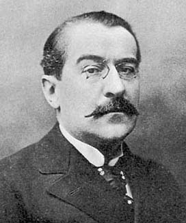
Existence of solutions to Differential Equations
Contents
The simplest case
If the right hand side of a differential equation does not contain the unknown
function then we can solve it by integrating: the solution of
\begin{equation}
\frac{dx}{dt} = f(t), \quad x(t_0) = x_0 \label{eq:simplest-ODE}
\end{equation}
is
\[
x(t) = x_0 + \int_{t_0}^t f(s) ds.
\]
This is just the fundamental theorem of calculus.
In calculus we learn a number of tricks that allow us to solve differential
equations with more complicated right hand sides. These tricks all involve some
manipulation of the differential equation that turns it into the simplest case
\eqref{eq:simplest-ODE}, so we can solve it by integrating. The most important
cases are separable differential equations and first order linear differential
equations. Click here for a review.
The existence and uniqueness theorems deal with the equations that we cannot
solve using calculus.
The general case
Consider the differential
equation
\begin{equation}
\frac{dx}{dt} = f(t, x), \quad x(t_0) = x_0
\label{eq:ODE}
\end{equation}
Assume the right hand side $f(t, x)$ in the
equation \eqref{eq:ODE} is a function of two variables that is
defined in the rectangle $R$ consisting of all $(x, t)$ with
\[
x_0-\delta \leq x \leq x_0+\delta, \quad t_- \leq t \leq t_+~~.
\]
The existence theorem.
Suppose the right hand side $f$ is bounded, i.e. assume that there is a
constant $M$ such that
\[
|f(t, x)|\leq M
\]
holds for all $x$ and $t$. Suppose also that $f$ satisfies the Lipschitz
condition, i.e. assume that there is a constant $L$ such that
\[
|f(t,
x) - f(t, y)| \leq L |x-y|
\]
holds for all $x, y$, and $t$. Then the differential equation \eqref{eq:ODE} has
a solution $x(t)$, which is defined on some interval $t_0-\epsilon \lt t \lt
t_0+\epsilon$ for some number $\epsilon\gt0$.
Proof by Picard iteration of the Existence Theorem
There is a technique for proving that a solution exists, which goes back to
Émile Picard (1856—1941).
 Here is a simplified version of his proof.
The (important) details follow
below.
Not knowing any solution to the ODE, we begin with a first
guess, namely $x_0(t) = x_0$. We try to improve on this guess by
solving
\[
\frac{dx_1}{dt} = f(t, x_0), \quad x_1(t_0) = x_0,
\]
which gives us a new function $x_1(t)$. The right hand side in
this differential equation only contains $x_0$, so it is known
and we can find $x_1(t)$ by integrating. The function $x_1(t)$
that we get is still not a solution of the ODE \eqref{eq:ODE}
that we want to solve, so we try to improve it again by solving
\[
\frac{dx_2}{dt} = f(t, x_1(t)), \quad x_1(t_0) = x_0,
\]
which
gives us another new function $x_2(t)$. Picard's idea was to
repeat this process infinitely often, which results in a sequence
of functions $x_0(t)$, $x_1(t)$, $x_2(t)$, $\cdots$, in which the
$n$th function is defined by solving
\begin{equation}
\frac{dx_n}{dt} = f(t, x_{n-1}(t)), \quad x_{n-1}(t_0) = x_0.
\label{eq:picard-iteration}
\end{equation} The key part of the
whole construction is to prove that the functions $x_k(t)$
converge, as $k\to\infty$, and that the limit
\[
x(t)
\stackrel{\rm def}= \lim_{k\to\infty} x_k(t)
\]
is a solution of the ODE.
This procedure of generating a sequence of functions which approximate
the solution whose existence we are trying to establish, is
called Picard iteration.
Details of Picard’s proof
Choice of $\epsilon$
We will choose
\begin{equation}
\epsilon = \min \Bigl\{ \frac1{2L}, \frac{\delta}{M} \Bigr\}
\label{eq:epsilon-choice}
\end{equation}
The reason for this choice will not become clear until later in the proof,
so for now we will simply write $\epsilon$ and not worry about its specific
value.
The $x_k(t)$ are well–defined
By definition we get $x_k(t)$ from $x_{k-1}(t)$ by solving
\eqref{eq:picard-iteration}, i.e. by integrating
\[
x_k(t) = x_0 + \int_{t_0}^t f(s, x_{k-1}(s))\; ds.
\]
Here we have to substitute $x_{k-1}(t)$ in the function $f(t, x)$. Since
this function is only defined for $x_0-\delta\leq x\leq x_0+\delta$ (as far
as we know), we have to be sure that $x_0-\delta\leq x_{k-1}(t) \leq
x_0+\delta$ holds for all $t$ with $t_0-\epsilon \le t \le t_0+\epsilon$.
For the first approximation $x_0(t)$ this is automatically
true since $x_0(t) = x_0$ is constant.
The second approximation $x_1(t)$ is a function whose
derivative is bounded by
\[
|x_1'(t)| = \bigl|f(t, x_0(t))\bigr|
\leq M,
\]
as we have assumed in the
theorem. Since $x_1$ is a function whose derivative is never
more than $M$, and since $x_1(0) = x_0$, it follows that for
$t_0-\epsilon \le t \le t_0+\epsilon$ one has
\[
\bigl| x_1(t) - x_0 \bigr| \leq M |t-t_0| \leq M\epsilon.
\]
Our choice of $\epsilon$ implies that
\begin{equation}
|x_1(t)-x_0|\leq \delta, \text{ i.e. }
x_0-\delta \le x_1(t) \le x_0+\delta \text { for }t_0-\epsilon
\le t \le t_0+\epsilon. \label{eq:x1bound}
\end{equation}
Therefore $f(t, x_1(t))$ is well–defined, and we can repeat the same
arguments: since $x_2'(t) = f(t, x_1(t))$ we have $|x_2'(t)|\leq M$, so
that $x_2(t)$ cannot change more than $M\cdot \epsilon$ during a time
interval of length $\epsilon$. Hence $x_2(t)$ also satisfies $x_0-\delta
\le x_2(t) \le x_0+\delta$ for as long as $t_0-\epsilon \le t \le
t_0+\epsilon$.
The difference $y_k$ between two successive approximations
The key to proving that the $x_k(t)$ converge is to estimate the difference
between two successive $x_k$’s. We define
\[
y_k(t) =
x_k(t)-x_{k-1}(t).
\]
If we know something about the $y_k(t)$ then we can go back to the functions
$x_k(t)$ by adding:
\[
x_k(t) = x_0 + y_1(t) + y_2(t) + \cdots + y_k(t).
\]
We will
measure the size of the terms $y_k(t)$ by means of
\[
m_k
\stackrel{\rm def}= \max _{t_0-\epsilon \le t \le t_0+\epsilon}
\left| y_k(t) \right|.
\]
An estimate for $m_1$
For $k=1$ we have $y_1(t) = x_1(t)-x_0$, and it
follows from \eqref{eq:x1bound} that $|y_1(t)|\leq \delta$. Hence
\begin{equation} m_1\leq \delta. \label{eq:m1bound}
\end{equation}
Estimating $m_k$ for $k>1$
Since both $x_k$ and $x_{k-1}$ satisfy the
same initial condition $x(t_0) = x_0$, we have
\[
y_k(t_0) =
x_k(t_0) - x_{k-1}(t_0) = x_0 - x_0 = 0.
\]
For the derivative of
$y_k$ we have
\[
\frac{dy_k}{dt} = \frac{dx_k}{dt} -
\frac{dx_{k-1}}{dt} = f\bigl(t, x_{k-1}(t)\bigr) - f\bigl(t,
x_{k-2}(t)\bigr)
\]
so that
\[
\left| \frac{dy_k}{dt} \right|
\leq L |x_{k-1}(t) - x_{k-2}(t)| = L |y_{k-1}(t)| \le Lm_{k-1}.
\]
Since $y_{k}(t_0) = 0$, this implies that for all $t$ in the
interval $(t_0-\epsilon, t_0+\epsilon)$ we get
\[
|y_k(t)|\leq
L\epsilon m_{k-1}.
\]
The maximal value of $|y_k(t)|$ therefore
also satisfies this inequality, so that we have
\[
m_k \leq
L\epsilon\cdot m_{k-1}.
\]
We now use \eqref{eq:epsilon-choice}
again, where we chose $\epsilon \leq 1/(2L)$. This choice implies
that $L\epsilon \leq \frac12$, so that
\[
m_k\leq \tfrac12
m_{k-1} \leq \bigl(\tfrac12\bigr)^2 m_{k-2} \leq
\bigl(\tfrac12\bigr)^3 m_{k-3} \leq \cdots \leq
\bigl(\tfrac12\bigr)^{k-1} m_{1} \leq \bigl(\tfrac12\bigr)^{k-1}
\delta.
\]
The series $\sum y_k(t)$ converges; the sequence
$x_k(t)$ converges
Since
\[
|y_k(t)|\leq m_k \leq
\bigl(\tfrac12\bigr)^{k-1} \delta,
\]
we have
\[
\sum_{k=1}^\infty |y_k(t)| \leq \sum_{k=1}^\infty m_k \leq
\sum_{k=1}^\infty \bigl(\tfrac12\bigr)^{k-1} \delta = 2\delta,
\]
by the geometric series.
Since the series $\sum |y_k(t)|$ converges, the series $\sum_k
y_k(t)$ also converges. Hence
\[
x(t) \stackrel{\rm def}=
\lim_{k\to\infty} x_k(t)= \lim_{k\to\infty}
x_0+y_1(t)+\cdots+y_k(t)= x_0+\sum_{k=1}^\infty y_k(t)
\]
exists—the sequence of functions $x_k(t)$ converges.
How fast does the sequence
converge?
The difference between the $k$th approximation $x_k(t)$ and the
limit $x(t)$ is
\[
x(t) - x_k(t) =
y_{k+1}(t) + y_{k+2}(t) + \cdots = \sum_{i=k+1}^\infty y_i(t).
\]
We can estimate it by
\[
|x(t) - x_k(t)| \leq \sum_{i=k+1}^\infty
|y_i(t)| \leq \sum_{i=k+1}^\infty
\delta\bigl(\tfrac12\bigr)^{i-1}
=\delta\bigl(\tfrac12\bigr)^{k-1}.
\]
So every approximation
$x_k$ should be about twice as accurate as the previous one.
Proving that the limit is a solution
We have shown that the functions $x_k(t)$ have a limit $x(t)$, but we still
have to show that this function satisfies the differential equation. We
reason indirectly by showing that the limit $x(t)$ satisfies an integral
equation, and then differentiating both sides of that equation. Here is the
computation:
\begin{align*}
x(t) &= \lim_{k\to \infty} x_{k+1}(t) \\
&= \lim_{k\to\infty} x_0 +\int_0^t f(s, x_k(s)) ds \\
&= x_0 +\lim_{k\to\infty} \int_{t_0}^t f(s, x_k(s)) ds\\
&= x_0 +\int_{t_0}^t \lim_{k\to\infty} f(s, x_k(s)) ds\\
&= x_0 + \int_{t_0}^t f(s, x(s)) ds.
\end{align*}
Therefore $x(t)$ is differentiable, and its derivative is
\[
\frac{dx}{dt} = f(t, x(t)).
\]
Sticky points
Picard's construction involves taking the limit of a sequence of functions. In
the proof we used the plausible looking “fact”
\[
\lim_{n\to\infty} \int_a^b f_n(t) dt =
\int_a^b \lim_{n\to\infty} f_n(t) dt,
\]
We also assumed that the limit function $x(t)$ is such that the integral
$\int_{t_0}^t f(s, x(s))\, ds$ is well defined as a Riemann integral. This kind
of question can be answered with some real analysis, in particular, by using the
concept of “uniform convergence” for a sequence of functions. We
will not address these points in this course.
 Here is a simplified version of his proof.
The (important) details follow
below.